
Pearson Correlation Coefficient.
In statistics, we like to summarize everything to a single number. Be it spread of the data, measure of central tendency or a 2d scatter plot. Because, few numbers are easier to analyse. Coefficient of correlation is one such number which summarizes scatter plot.
Correlation Coefficient- $r$
It is a number ranging from $-1$ to $1$ which determines the degree of linear relationship/correlation between two variables. In other words, it determines how well we can plot the data points generated by two variables on a single line. It can also tell us the slope of the line which can be fit to this data. Let’s first try understand how to interpret the coefficient of correlation $r$.
Given two variables $x$ and $y$, there are three possibilities in terms of linear correlation.
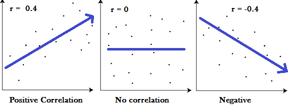
- When $y$ increases with $x$, positive correlation
- When $y$ decreases with $x$, negative correlation
- When $y$ does not change with respect to $x$, no correlation
 |
|---|
| Credit: StatisticsHowTo |
Yoe can see all three cases in the figure above. The figure shows scatter plot of points $(x,y)$ for three different condition. Notice, when the $y$ is increasing with $x$ the value of $r$ is positive and when it is decreasing with $x$ the value of $r$ is negative. Also, in figure with no correlation, you can not find any straight line which can summarize the trend in the data, making the value of $r$ zero.
If the value of $r$ was $1$, the conclusion would be, all the points in the scatter plot are on the same line which has a positive slope. If the value of $r$ is $-1$, all the points in the scatter plot are on the same line with negative slope. Values closer to 1 or $-1$ depicts a strong correlation. Whereas values, closer to 0, depicts a weak correlation.
How to calculate the Pearson Correlation Coefficient - $r$:
It is mean product of $z$-scores of the two variables. That means, calculate $z$-scores of the two variables, multiply theme element wise and take average of them.
\[\begin{aligned} r = \frac{1}{n-1}\sum_{i=1}^{n}zx_i.zy_i \end{aligned}\]Where,
$n$ = number of elements in the sample,
$ zx_i $ = $ z $-score of $i^{th}$ element of $x$,
$ zx_i = \frac{x_i-\bar{x}}{s_x}$,
$s_x$ being standard deviation of $x$,
$zy_i$ = $z$-score of $i^{th}$ element of $y$,
$ zy_i = \frac{y_i-\bar{y}}{s_y} $,
$s_y$ being standard deviation of $y$
This equation can be further solved but I find above version easy to remember and intuitive. Let’s substitute values of $z$-scores $(zx_i, zy_i)$ and standard deviations $(s_x, s_y)$ in above equation.
\[\begin{align} r &=& \frac{1}{n-1}\sum_{i=1}^{n}\frac{(x_i-\bar{x})(y_i-\bar{y})}{s_x.s_y} \\\\ &=& \frac{1}{n-1}\sum_{i=1}^{n}\frac{(x_i-\bar{x})(y_i-\bar{y})}{\sqrt{\frac{(x_i-\bar{x})^2}{n-1}}.\sqrt{\frac{(y_i-\bar{y})^2}{n-1}}} \\\\ &=& \sum_{i=1}^{n}\frac{(x_i-\bar{x})(y_i-\bar{y})}{\sqrt{\sum_{i=1}^{n}{(x_i-\bar{x})^2}}.\sqrt{\sum_{i=1}^{n}{(y_i-\bar{y})^2}}} \end{align}\]Why it works:
The product, $ (zx_i*zy_i) $ is positive iff $x_i$ and $y_i$ both are either simultaneously less than or simultaneously greater than their respective means making the resulting $r$ positive. Similarly, the product $ zx_i*zy_i $ is negative iff $x_i$ and $y_i$ have opposite relationship with their respective mean, i.e, either $(x_i > \bar{x})\text{ & }(y_i < \bar{y})$ or $(x_i < \bar{x}) \text{ & } (y_i > \bar{y})$, making the resulting $r$ negative. The absolute value of $r$ is larger when either of the tendency is stronger.
And that’s it.